Autodifferentiation

Having a deep understanding of autodifferentiation (AD) is essential for deep learning research, but this is not obvious. Backpropagation (a specialized subset of AD) is a developed field with its detailis often abstracted away from deep learning practitioners. Backpropagation is a leaky abstraction (Chekhov's footgun), and you should understand it. We're seeking to have a deeper than surface level understanding of these complex, powerful systems. The objectives for this post are as follows:

• Provide relevant background on derivatives, loss functions, and gradient descent
• Understand forward- and reverse- autodifferentiation
• Write some custom gradient operations in PyTorch.
• Describe optimal Jacobian accumulation
• Optional: learn how JAX derives reverse-mode autoderivatives by combining partial evaluation, forward-mode-autodifferentiation, and transposition.
• Optional: why is the computation of a divergence computationally expensive using autodifferentiation? Learn Hutchinson’s trace estimator. (Why is that efficient?) Learn the Hutch++ trace estimator. (Which is surprisingly poorly known.)

What is a derivative?

Calculus is usually one of the harder math classes you'll encounter either in high school or college. It's the omnipresent course standing between you and your dream job. Many dread it, some enjoy it. Calculus is the study of how things change with time as well as how to find the area of certain objects. It's a new way of thinking about the world and often requires robust visualization skills. Many people who aren't STEM majors wonder why it's typically a general education requirement. My best answer to that question is this: humans have trouble intuiting complex functions (particularly exponential ones) and such functions exist all around us. We experience the world as a series of static snapshots. We have a natural intuition about linear rates of change. However, many of the functions we encounter in life aren't as simple as your typical y = mx + b.

Imagine you're driving on the highway. Your speedometer shows you your instantaneous speed (or rate of change of position). If your speed is equal to the other cars around you and it is constant, all is well. However, if someone in front of you slams on the breaks, decelerating to a stop, you are hit with a pop quiz. How much distance is between your car and theirs? How quickly is that distance changing? How fast are you going? How quickly can you slow down? If you swerve into the next lane, will the other drivers have enough time to anticipate your presence and adjust accordingly? Luckily for us, most of the time we are able to make these judgement calls. However, if we fail this pop quiz, we could pay with our health.

"Speed has never killed anyone. Suddenly becoming stationary, that's what gets you."
-- Jeremy Clarkson

Think about the following examples: timing the stock market by estimating the rate of change of technology, and taking out loans with compound interest. Those who mistake exponentials for linear functions fare much worse that those who see the patterns for what they are. Derivatives are fundamental to everyday life, as well as numerous areas of specialization.

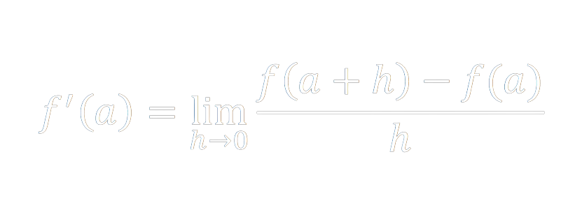
A derivative is the rate of change of a function. Graphically, imagine taking two points on a curve and extending a line through them. This line is the average rate of change of your function over that interval. Then take one point, and iteratively nudge it closer and closer to the other (updating your intersecting line at each step) until the distance between them is infinitesimally small. The final tangent line represents the instantaneous rate of change of your function at the point in question.

Why do we care about derivatives in the context of Machine Learning?

In ML we have to have a concrete metric to define the performance of our model. This metric is typically called the loss function, cost function, or objective function. An intuitive candidate for a loss function of a classification model would be this:

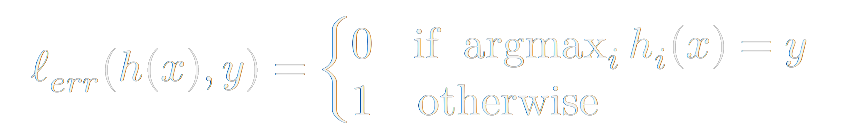
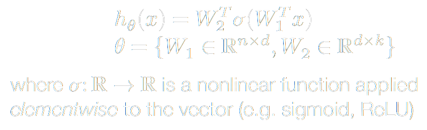
This is a perfect measure for the accuracy of a classifier. However, we would like a function that is more amenable to optimization. We will talk more why in a second, but we would much rather prefer a differentiable function. Let's take a step back and think about our inputs and outputs. As we train our model, we take an example vector (say, an image) input it into our model, then the model does it's magic. Well, what is this magic? The model attempts to learn a hypothesis function h(x) (i.e. a transformation that uses a linear operator such as matrix multiplication – in neural networks, a series of parameterized nonlinear functions are thrown into the mix) that maps our n-dimensional data-space to our k-dimensional class-space.

Our model outputs a vector of probabilities rather than a single discrete prediction per example. Each index of that vector corresponds to a class (i.e. category). The output vector index with the highest value is the class that our model believes the example most likely belongs to. Speaking of the output vector: our hypothesis function maps to set real numbered k-dimensional vectors (R^k) ({h(x): Rⁿ -> R^k }). Whereas, we normally think of probabilities as floats between 0 and 1 inclusive, such that the sum of the probabilites of the set of possible events equals 1 (more formally, we want to add constraints to the elements h_i of h(x): {h(x): Rⁿ -> R^k | 0 <= h_i <= 1; Σ h_i = 1}). To get this behavior, we can apply the softmax function to the output of our hypothesis function:

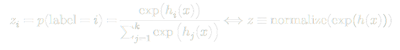
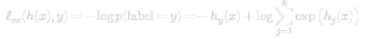
From there, we can define a commonly used loss function. By convention, we would like to minimize the loss. However, if the quantity we are dealing with is the probability that we guessed right, higher is better. As you may have seen in a Linear Programming course, we can change a maximize problem into a minimize problem by negating it. Additionally, because minimizing probabilities is poorly conditioned numerically, we will take the logarithm of our probabilities first. Giving rise to the Negative Log loss.

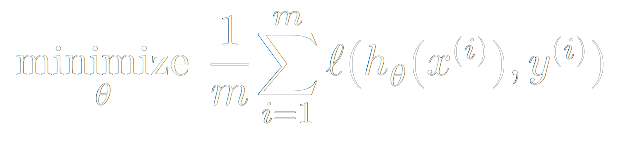
Our problem then becomes simple: how do we minimize the average loss on our training set? Which values of our parameters θ, W (i.e. the entries of the matrices we multiply our input vector by) provide the best results? That is,

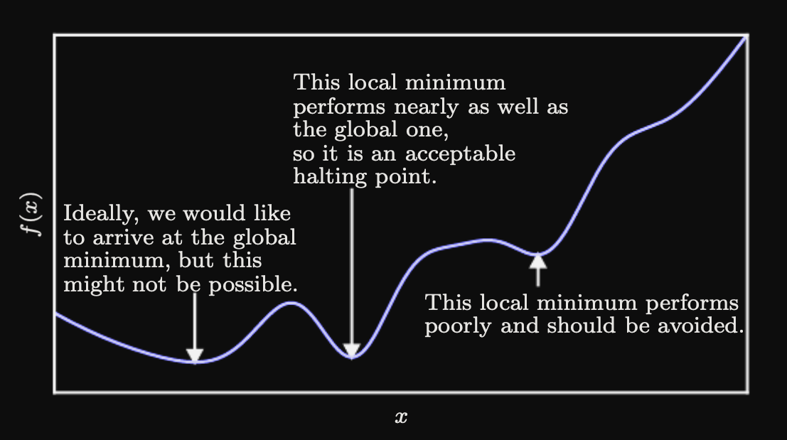
Just like any other function we can graph this and look at the resulting curve. On the x-axis we have our independent variable (aka our parameter or the knob that we can tune) and on the y-axis we have our dependent loss value. Since our loss function is a measure of how inaccurate our model is, we want to minimize the loss value. When we imagine the derivative of our loss function for a particular x-value, it points in the direction of rate of change. Are we getting better at making predictions (are we learning?) or are we getting worse? We are looking for a minima of the loss function. So if our derivative is negative, we should go in that direction. Extrema (maxima or minima) occur whenever the derivative equals zero. Whenever the derivative changes from negative to positive (given we're traversing the curve in the direction of increasing x values), we've passed over a minima of the function and that tells us this might be a good place to stop.  The derivative acts as our compass in determining the best x values to pick.

We have made a big simplification for visualization sake: in machine learning contexts we typically have millions to billions of independent variables – knobs (aka weights or parameters) that we can turn. While it is difficult to visualize n-dimensional space (where n > 3), 3-D is a good enough proxy to understand the concepts. The notion of the derivative intuitively extends into arbitrary dimensional space, giving rise to partial derivatives. The partial derivative of a function with respect to a particular variable is the derivative of the function, holding all other variables constant. The set of partial derivatives of a function is called the gradient of that function. Because our variables are already organized into a matrix, we can correspondingly organize the gradient into a matrix. By convention, the gradient always points in the rate of maximum increase. Therefore a corollary of our previous loss minimizing heuristic is to always move in the opposite direction of the gradient – giving rise to the technique known as Gradient Descent.

To alter our weights in a way that moves our predictions in the opposite direction of the gradient, we can update it by decrementing it by some multiple of the gradient. The factor we multiply the gradient is called the learning rate. When choosing a learning rate, we want a value that doesn't take forever for the loss to converge, but also doesn't make it bounce all over the place and overshoot the optimal weights. It often makes sense to decrease as our learning rate model runs a specified number of times. This process is called learning rate decay.  

Generally in Machine Learning, the more data you have, the better your results could be. But often times this means that our dataset cannot fit in our computer's memory. Therefore we have to break the data down into more manageable subsets. We also try to take advantage of the parallelism found in modern GPUs. For these reasons, we process several examples simultaneously in batches. These batches are randomly selected to ensure that each batch is as representative of the underlying data distribution as possible. Performing iterated gradient descent on these minibatches is referred to as Stochastic Gradient Descent.

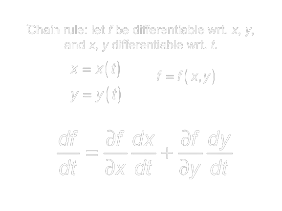
We've covered the case for a single function's gradient and how it can be used to minimize loss. What happens when we compose (i.e. chain) many functions, each containing their own independent weights together? If you have taken Calculus you've likely encountered the Chain rule at some point in time. It may have been a while since you've seen it so let's go over it briefly. Let's say you want to figure out how a function f changes with respect to some variable t. However f is composed of two functions x and y, each of which are functions of t. There are four things we have to know in order to answer our question: how t affects x , how t affects y, how x affects f and lastly, how y affects f. The Chain rule says that we can multiply x's influence on f with t's influence on x, and do likewise with y, summing the two to complete the derivative. Using the formula below, we can break down our original problem into more approachable pieces.

How do we actually find derivatives in practice?

There are four ways to do so:

1) Manually working them out (the way you learn in Calculus class) and hard coding them (e.g. if f(x) = 3x² + e^2x , then f'(x) = 6x + 2e^2x )

2) Numerical differentiation using finite difference approximations (Like we mentioned when taking the two dots arbitrarily close to one another) – this is actually used in unit tests to check implementations of #4

3) Symbolic differentiation via expression manipulation (as you may have used in online wolfram-alpha style derivative calculators)

4) Automatic Differentiation (AD) which we will focus on in this post

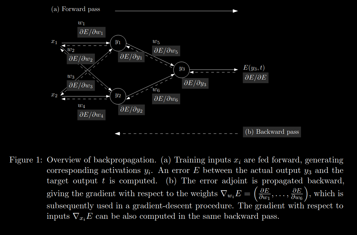
Automatic Differentiation "compute[s] derivatives through accumulation of values during code execution to generate numerical derivative evaluations rather than derivative expressions" [here's where I got the quote from, it's also a great in depth AD reference]. Let's translate that into more of layman's terms. AD is similar to how compilers create directed graphs to model the internal representations of the program being compiled. During AD, a computational graph is created. This graph essentially bookkeeps the relationships of various functions to one another throughout our neural network so that we can know how to properly apply the chain rule later on.

When an operation is performed, a new tensor is created. A mathematical tensor is a higher dimensional matrix, think of going from one face of a rubix cube to the entire cube (or a hypercube for higher order tensors). After creating the new tensor, AD notes the tensors that played a part in it's creation. AD then uses this information to get the gradient of the tensor with respect to each of its parent tensors.

There are two primary 'modes' of AD: forward and reverse.

In forward-mode autodifferentiation, the computational graph is traversed from the leaf nodes to the root node. In reverse-mode autodifferentiation, the opposite is done. Which AD mode you choose determines the direction in which you recursively traverse the chain rule. While the distinction seems trivial, there are certain classes of functions for which one mode is more equivalent than the other. It depends on the dimensionality of the function's input-space to it's output-space. The larger the disparity between the two, the greater the potential efficiency gains in choosing a particular mode.  

Backpropagation as utilized in many modern deep learning frameworks such as Pytorch is a special case of reverse-mode autodifferentiation. This choice of mode makes sense because, in Machine Learning, we are trying to find efficient embeddings that map our high dimensional data-space to a more informative lower dimensional inference-space. E.g. mapping Rⁿ -> R^k where n >> k.

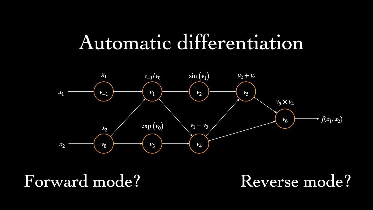
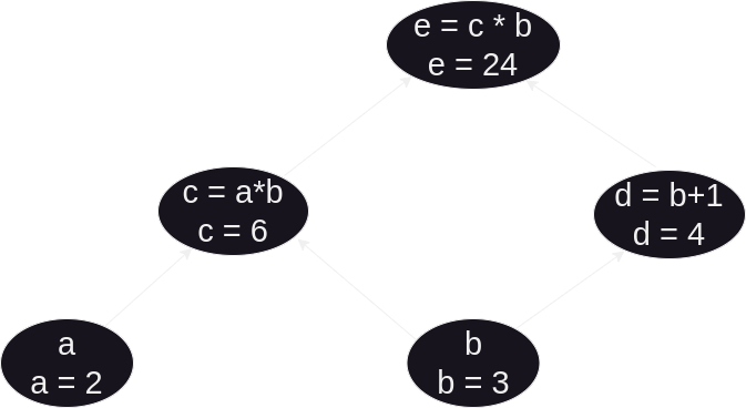
For example's sake, let's take a look at forward-mode autodifferentiation since it is little more natural to compute. Let's say, for example we have a function e defined by e = (a*b) * (b+1). As we can see, e is the product composition of two intermediate functions c = (a*b) and d = (b+1). Let's initialize these values (setting a = 2 and b = 3) and graph their relations – each function becomes a vertex, and the connecting edges represent dependencies (where a function is used in the future).

The function we care about is e, but the only direct control we have over e is through the initial variables a and b. What we want to know is, if we alter a or b what kind of changes can we expect to see in the value of e? To do this, we need to utilize the chain rule, as well as the sum rule and product rule. Yielding to the rigor behind their definitions, there are two easy heuristics one can follow. Regarding the sum rule, the derivative of the addition operation is always 1. Likewise, the derivative of the product operation with respect to one operand is the other operand (or product of other operands if more than one).

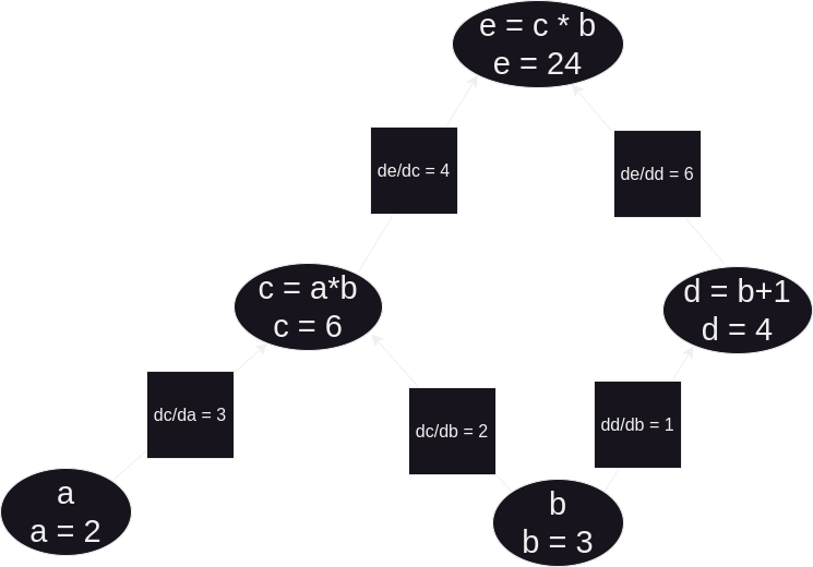
So, now we can finally answer our question. How does e change in response to a, and likewise to b? The derivative of e with respect to a: ∂e/∂a = ∂e/∂c * ∂c/∂a. Or when plugging in the numbers for our above example, ∂e/∂a = 4 * 3 = 12. Secondly, the derivative of e w.r.t. b: ∂e/∂b = (∂e/∂c * ∂c/∂b) + (∂e/∂d * ∂d/∂b). Or, concretely, ∂e/∂b = (4 * 2) + (6 * 1) = 14. Therefore, by comparing these partial derivatives, we can see that e grows fastest by increasing b (and conversely shrinks fastest by decreasing b).  

Again, we have made another simplification for pedagogy's sake. Our vertices are not scalars and scalar functions – instead, they are matrices, matrix products, and pointwise nonlinear functions. When calculating the partial derivatives of matrices with respect to other matrices, we get into the wonky world of matrix differential calculus. For the sake of this blog-post we will hand-waive over this and instead stick with this more hacky way to derive our gradients. What we do is, pretend everything is a scalar, use the chain rule, and then rearrange/transpose your matrices to make the sizes work (verifying your answer numerically). I would go down the rabbit hole of how to manually derive the gradients of real loss functions, but it is infeasible for modern models, and our time might better be spent focusing on how we can programmatically do it.

What does the Reverse-Mode AD algorithm look like?

Placeholder

An Important Scenario to be Aware Of:

Almost all operations are differentiable. The requirements for differentiability are 1: the function should be continuous and defined for all inputs, 2: the function should be smooth (no sharp corners), and 3: the function should map one input to only one output. Nearly all of the operations one might want to include in their neural network is differentiable, and I won't bore you with a list of their derivatives. However, one important caveat is what happens when you apply some common nonlinearities such as the sigmoid function.

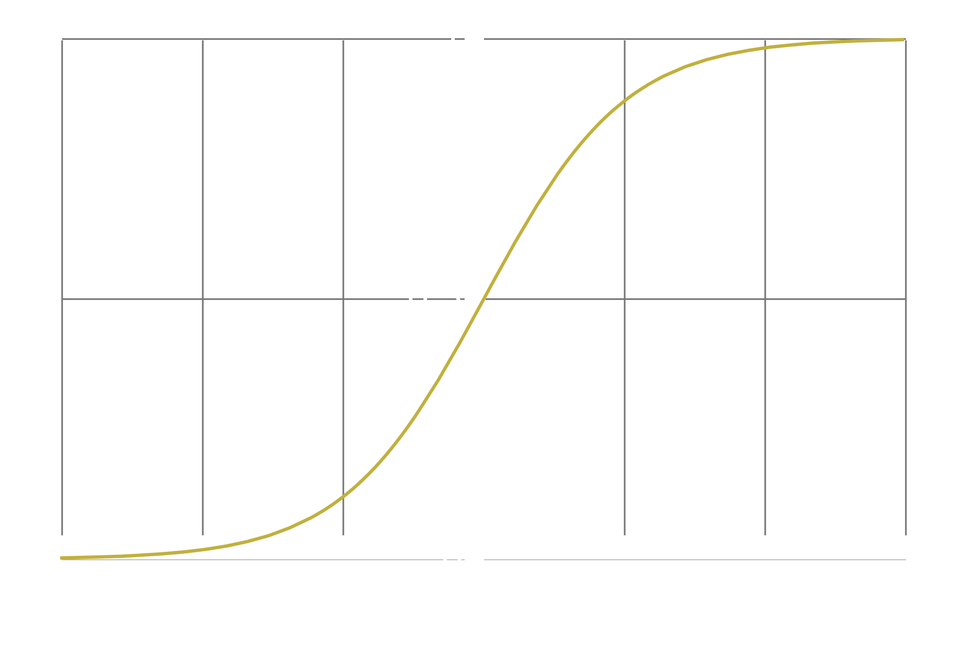
Pay attention to what happens at the tails of the function, as the input approaches infinity or negative infinity. The curve gradually gets flatter and flatter, asymptotically approaching 1 or -1 respectively. As we discussed previously, when a curve is flat, the derivative of the curve at that point is equal to 0. While, in the literal sense of the word, the sigmoid is never truly flat, it is asymptotically flat, which is a problem. Since computers only have a finite memory, they can only approximate decimal numbers to a limited accuracy. An implication of this is that if a number becomes too small, the computer cannot represent it accurately and instead rounds it down to 0. This is called numerical underflow. This is a problem because if a neuron has extreme values, and we apply the sigmoid nonlinearity to that neuron's layer, that said neuron's derivative will be set to 0. If the neuron's derivative is set to 0, backpropagation will assume that there is no use in altering it, since it seems to have no impact on the loss function. From that point on, this neuron is essentially brain dead.

This can be counteracted by applying batch normalization to that layer. Normalization is a way to scale down a tensor so that the outliers are less extreme, but also such that the original ratios of elements to one another are preserved. Batch normalization is a way to normalize all tensors across a batch simultaneously. We will not go into the details of how this is performed due to space constraints, but it is essential to be aware of it's presence and when to use it.

The astute reader might have noticed that by finding all the partials down a subgraph of our graph is similar to the gradient idea we explored earlier. However, instead of dealing with one function's gradient, we are dealing with the gradients of several functions. A different way to compile all these different partial derivatives is to organize them into a sort of lookup table – a tensor that we call the Jacobian. As you can see in the image below, the Jacobian is simply the concatenation of all the gradients of all the composite functions of your subject function. Each row represents a particular function and each column represents a particular variable that we are differentiating that function with respect to.

When we perform AD in the context of Machine Learning, we are computing the Jacobian of the Loss function. As we stated earlier, we choose reverse-mode AD because it tends to be slightly more efficient in our use case. However, there are several other ways to perform AD. The general problem of finding a function's Jacobian in the most efficient manner possible is called the Optimal Jacobian Accumulation problem and is NP-complete.  

To illustrate what's going on behind the scenes we'll pull some examples from Andrej Karpathy's awesome Neural Networks: Zero to Hero series and derive some gradients by hand to get a better idea for what AD is doing. In the following snippets we are defining a neural network in Pytorch.

n_embd = 10 # the dimensionality of the character embedding vectors
n_hidden = 64 # the number of neurons in the hidden layer of the MLP

g = torch.Generator().manual_seed(2147483647) # for reproducibility
C  = torch.randn((vocab_size, n_embd),            generator=g)
# Layer 1
W1 = torch.randn((n_embd * block_size, n_hidden), generator=g) * (5/3)/((n_embd * block_size)**0.5)
b1 = torch.randn(n_hidden,                        generator=g) * 0.1 # using b1 just for fun, it's useless because of BN
# Layer 2
W2 = torch.randn((n_hidden, vocab_size),          generator=g) * 0.1
b2 = torch.randn(vocab_size,                      generator=g) * 0.1
# BatchNorm parameters
bngain = torch.randn((1, n_hidden))*0.1 + 1.0
bnbias = torch.randn((1, n_hidden))*0.1

# Note: I am initializating many of these parameters in non-standard ways
# because sometimes initializating with e.g. all zeros could mask an 
#incorrect implementation of the backward pass.

parameters = [C, W1, b1, W2, b2, bngain, bnbias]
print(sum(p.nelement() for p in parameters)) # number of parameters in total
for p in parameters:
  p.requires_grad = True

The forward pass is verbosely broken down into it's atomic chunks to give us some extra practice.

# forward pass, "chunkated" into smaller steps that are possible to backward one at a time

emb = C[Xb] # embed the characters into vectors
embcat = emb.view(emb.shape[0], -1) # concatenate the vectors
# Linear layer 1
hprebn = embcat @ W1 + b1 # hidden layer pre-activation
# BatchNorm layer
bnmeani = 1/n*hprebn.sum(0, keepdim=True)
bndiff = hprebn - bnmeani
bndiff2 = bndiff**2
bnvar = 1/(n-1)*(bndiff2).sum(0, keepdim=True) # note: Bessel's correction (dividing by n-1, not n)
bnvar_inv = (bnvar + 1e-5)**-0.5
bnraw = bndiff * bnvar_inv
hpreact = bngain * bnraw + bnbias
# Non-linearity
h = torch.tanh(hpreact) # hidden layer
# Linear layer 2
logits = h @ W2 + b2 # output layer
# cross entropy loss (same as F.cross_entropy(logits, Yb))
logit_maxes = logits.max(1, keepdim=True).values
norm_logits = logits - logit_maxes # subtract max for numerical stability
counts = norm_logits.exp()
counts_sum = counts.sum(1, keepdims=True)
counts_sum_inv = counts_sum**-1 # if I use (1.0 / counts_sum) instead then I can't get backprop to be bit exact...
probs = counts * counts_sum_inv
logprobs = probs.log()
loss = -logprobs[range(n), Yb].mean()

# PyTorch backward pass
for p in parameters:
  p.grad = None
for t in [logprobs, probs, counts, counts_sum, counts_sum_inv, # afaik there is no cleaner way
          norm_logits, logit_maxes, logits, h, hpreact, bnraw,
         bnvar_inv, bnvar, bndiff2, bndiff, hprebn, bnmeani,
         embcat, emb]:
  t.retain_grad()
loss.backward()
loss

# Exercise 1: backprop through the whole thing manually, 
# backpropagating through exactly all of the variables 
# as they are defined in the forward pass above, one by one

dlogprobs = torch.zeros_like(logprobs)
dlogprobs[range(n), Yb] = -1.0/n
dprobs = (1.0 / probs) * dlogprobs
dcounts_sum_inv = (counts * dprobs).sum(1, keepdim=True)
dcounts = counts_sum_inv * dprobs
dcounts_sum = (-counts_sum**-2) * dcounts_sum_inv
dcounts += torch.ones_like(counts) * dcounts_sum
dnorm_logits = counts * dcounts
dlogits = dnorm_logits.clone()
dlogit_maxes = (-dnorm_logits).sum(1, keepdim=True)
dlogits += F.one_hot(logits.max(1).indices, num_classes=logits.shape[1]) * dlogit_maxes
dh = dlogits @ W2.T
dW2 = h.T @ dlogits
db2 = dlogits.sum(0)
dhpreact = (1.0 - h**2) * dh
dbngain = (bnraw * dhpreact).sum(0, keepdim=True)
dbnraw = bngain * dhpreact
dbnbias = dhpreact.sum(0, keepdim=True)
dbndiff = bnvar_inv * dbnraw
dbnvar_inv = (bndiff * dbnraw).sum(0, keepdim=True)
dbnvar = (-0.5*(bnvar + 1e-5)**-1.5) * dbnvar_inv
dbndiff2 = (1.0/(n-1))*torch.ones_like(bndiff2) * dbnvar
dbndiff += (2*bndiff) * dbndiff2
dhprebn = dbndiff.clone()
dbnmeani = (-dbndiff).sum(0)
dhprebn += 1.0/n * (torch.ones_like(hprebn) * dbnmeani)
dembcat = dhprebn @ W1.T
dW1 = embcat.T @ dhprebn
db1 = dhprebn.sum(0)
demb = dembcat.view(emb.shape)
dC = torch.zeros_like(C)
for k in range(Xb.shape[0]):
  for j in range(Xb.shape[1]):
    ix = Xb[k,j]
    dC[ix] += demb[k,j]