Convoluted Computation

What are some ways to combine functions (or set of numbers), say 'f(x)' and 'g(x)' to get a unique resulting function 'h(x)'? Some intuitive combinations would be to add the functions together (i.e. h(x) = f(x) + g(x)) or to multiply them (i.e. h(x) = f(x)g(x)). There is another way to compose two functions that is less commonly known called the convolution of said functions. The convolution operation (denoted by the asterisk *) is defined as follows:

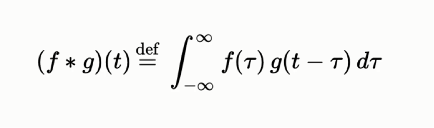
Convolutions often appear in signal processing, probability, differential equations, and when multiplying two polynomials. While those are all fascinating applications, we'll focus on the application of convolutions in image processing via Convolutional Neural Nets and cover the Winograd Convolution while we're at it.

In our use case, instead of functions as we typically define them, we will convolve two matrices. We can do this because a matrix represents a linear transformation (a function). The first matrix being our example image, and the second being a special matrix called a kernel (or filter). Let's say we would like to blur an image. For simplicity's sake, let's assume our input is a square 100 by 100 pixel image, and we want to use a 5 by 5 kernel. When calculating the pixel value at index [i, j] of our blurred image, we go to the [i, j]th position of our input image matrix, then we lay our kernel on top, aligning the center (index [3, 3]) of our kernel with our current position. We will call this overlap of kernel and image our receptive field. From there, the output pixel value of the given position is the sum of the corresponding point-wise products of our kernel and image matrices. For an ideal blur, we could choose to sample our kernel values from a Gaussian (normal) distribution as such:

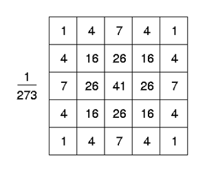
Thus we would give the current pixel index [i, j] the most weight in determining our output, and taper down the weight of a given position within the receptive field proportionally to the distance. After a given index is processed, the kernel slides one unit to the right – or if it reaches the edge of the image it starts on the next line down – and does it again. This (hopefully) makes sense, but the astute reader would be concerned about the (literal) edge cases – what happens for the positions where the kernel would be hanging off the side of the image? For that we utilize what is called padding. Padding is the arbitrary concatenation of pixels on the edge of an image to make the numbers work. As far as what values to put in the padded section there are several options, but for this case it makes the most sense to match whatever our boundary pixels are. While this does give the edge pixels more weight in determining the blurred pixel, close is often good enough and we'll consider that a cheap cost of being able to legally process arbitrarily sized images.

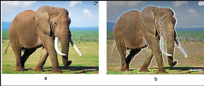
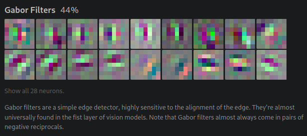
Ok, so far so good. You can create more and more complicated kernels that filter the image in more interesting ways. We could extend this idea of using the neighboring context around a pixel (with Gaussian sampling) to determine where there is a large variation between a pixel and its neighbors. Think of an image of a beach landscape. Half of the image is blue from the sky, but all of a sudden at the horizon, there is a shift in color from blue to a tan sandy color. The type of filter that is good at detecting those sort of sudden changes is called a Gabor filter (GF). Gabor filteres are special, as they have been shown to almost universally appear in the first layer of vision models.

Any particular Gabor filter kernel detects changes in a particular direction (e.g. left to right, bottom to top, etc.). Therefore, since (again) matrices are linear transformations, we can compose several GFs of the same orientation, with different phases to get the complex GF that can detect stripes. Or we can compose a complex GF with an orthogonal complex GF to get a "hatch" detector. Or we can similarly compose several Gabor filters of varying orientations in a piecewise fashion to get line detectors, curve detectors, corner detectors, divergence detectors, and even circle detectors. Linear combinations of the set of all the Gabor filter variants covering 180 degrees are invaluable in generalized detections of edges. (Note: not 360 because variance from left -> right is equivalent to variance from right -> left, hence a GF is its own negative reciprocal). At this point it becomes easy to see how useful this sort of kernel becomes when approaching image segmentation tasks.

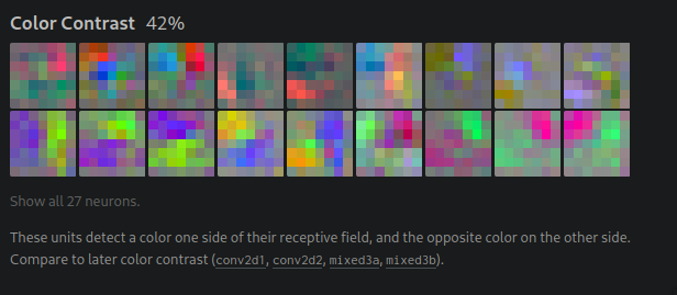
Another primitive type of kernel is the Color Contrast filter. This sort of kernel tries to detect cases in which one side of the receptive field is the opposite color as the other side. This can be useful for image classification. Imagine, we were trying to identify spiders. Let's suppose we already know how to identify the general shape of a spider. From that point on, a lot of vital information is conveyed by the spider's color. But we brushed over a valuable piece of the puzzle. How do we get from complex linear combinations of Gabor filters to full fledged object classifiers?

Edges tend to define curves. Think of a face, it is an oval, containing two lines for eyebrows, two circles below those lines for eyes, and below that there's usually two lines with two circles for the nose, and so on. You could create kernels that are really good at identifying any of those particular features. Because, again, matrices represent linear transformations, we can compose of those several kernels to get a single model. Boom! Computer vision = solved... We can enumerate all the ways our brain validates whether we are looking at a face, then create kernels for each factor. Right?

Sadly, images can be really complicated. We don't give our visual cortexes enough credit. Andrej Karpathy did a great job of explaining why this approach does not scale. I won't regurgitate his words, but I would definitely recommend checking that post out, it's a short read. On a higher level, this is yet another example of the bitter lesson.

"[T]he actual contents of minds are tremendously, irredeemably complex; we should stop trying to find simple ways to think about the contents of minds... They are not what should be built in, as their complexity is endless; instead we should build in only the meta-methods that can find and capture this arbitrary complexity. Essential to these methods is that they can find good approximations, but the search for them should be by our methods, not by us.
-- Rich Sutton

In a way, this is what deep learning and the notion of Software 2.0 is all about. Computers are really freaking fast. We need to focus on methods that scale well and leverage that fact. We may not be able to hand-code all the kernels necessary, but we are on the right track. Why don't we just allow a neural network to learn the kernels instead?

That's exactly what computer vision models do. Neural networks have a reputation for being black boxes, and for a long time no one talked about neuron-club. Except for a few researches who chose to work on ways to better understand these models, coalescing into a field called interpretability research. Computer Vision (CV) is a special field, because we humans rely so heavily on our own vision, we have developed really robust recognition and pattern matching skills. Because of this, interpretability is much more easily tractable in CV models. If you would like to do a deep dive on reverse engineering a computer vision neural network, check out this article series from a series of researchers at some of the most prolific AI labs across the world. I'll share a few of the visualizations they've produced, as they're really neat to check out. But I'd really recommend you check out those articles, they go into a level of depth I could only dream of going into.

First, a note on how these feature visualizations and categorizations were created. Once we train a neural network, we end up with a set of weights. These weights, unfortunately cannot just be plotted and visualized in any meaningful fashion. One round-about way that we can do this is through starting with a random, noisy image. Then, we can take our trained model and focus on particular neurons, or layers of neurons. We can observe how often these neuron's fire, and then reverse engineer the noisy image to optimize for how frequently those neurons fire. By doing so, we can get an idea for what sort of images these neurons like. If we need more clues to explain a neuron family, we can observe the sets of example images for which these neurons fire with high confidence, as well as previous and future neurons with strong connections to these neurons.

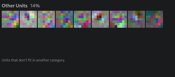
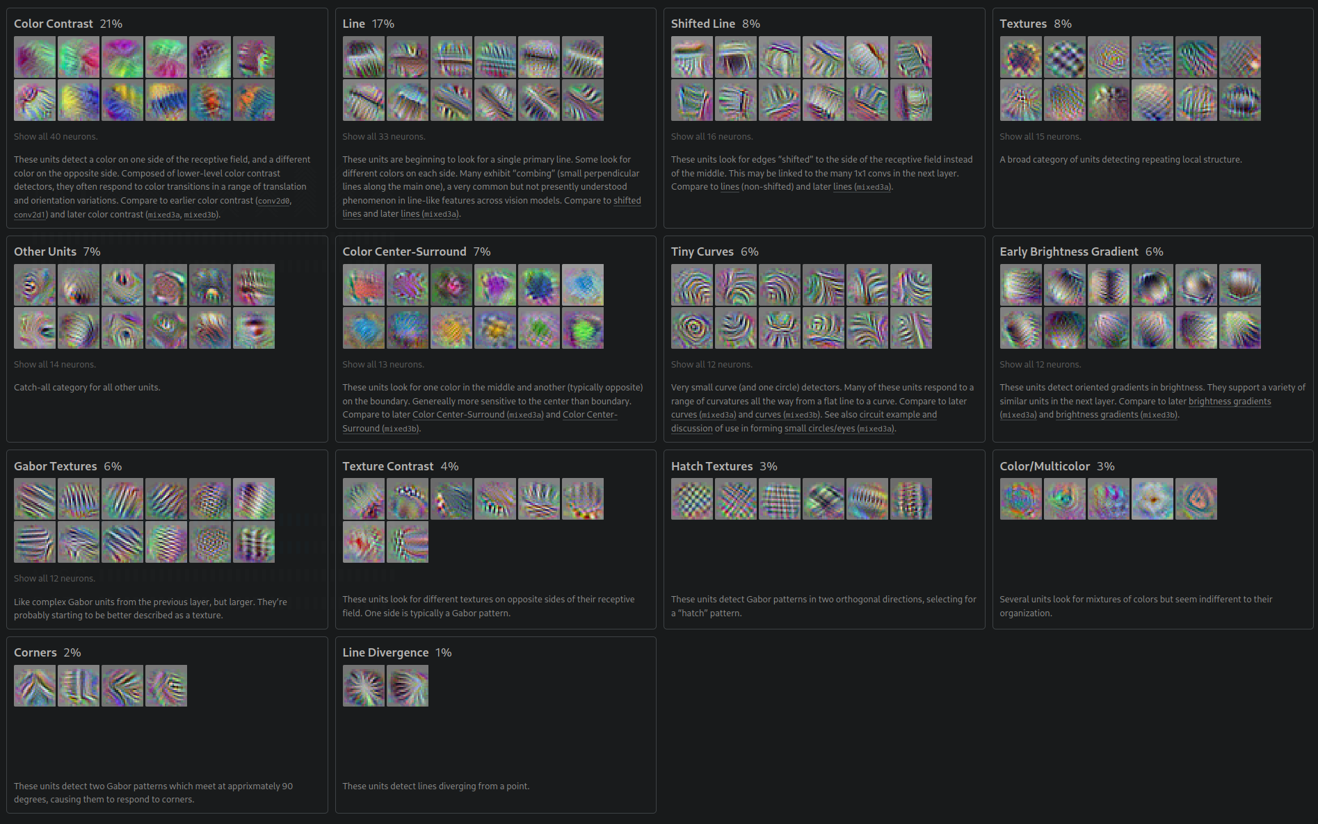
In the first convolutional layer of the Google's CNN Inception V1, you see filters like the following:

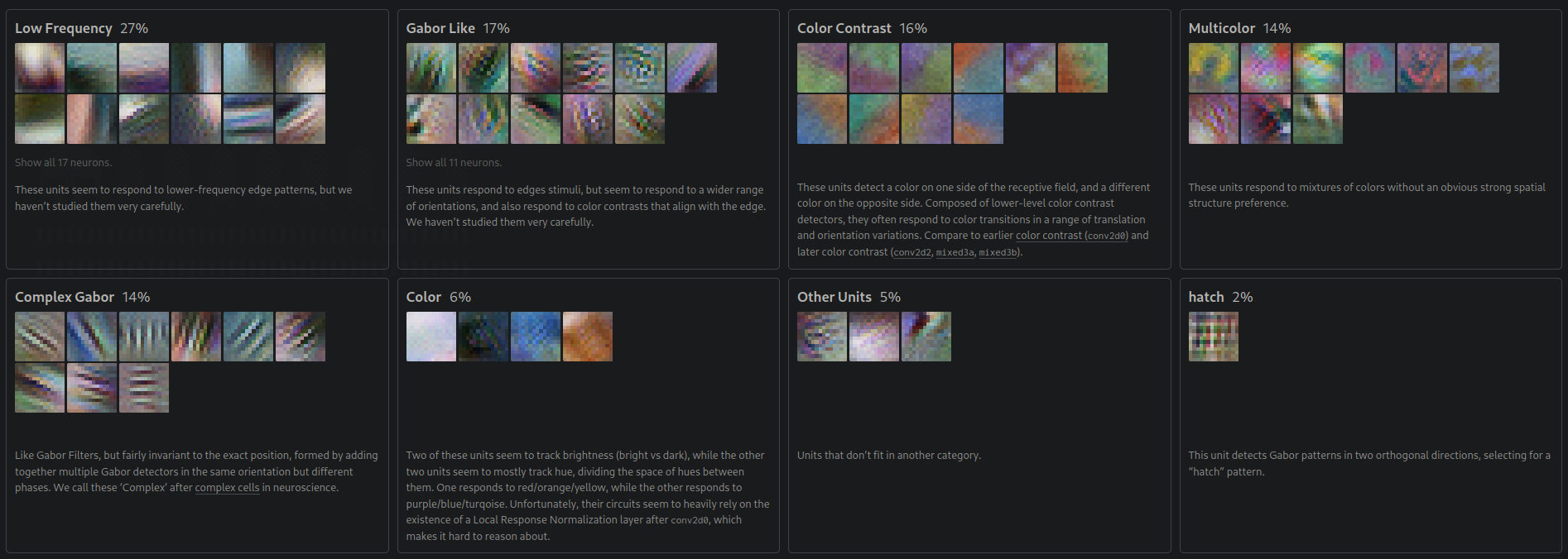
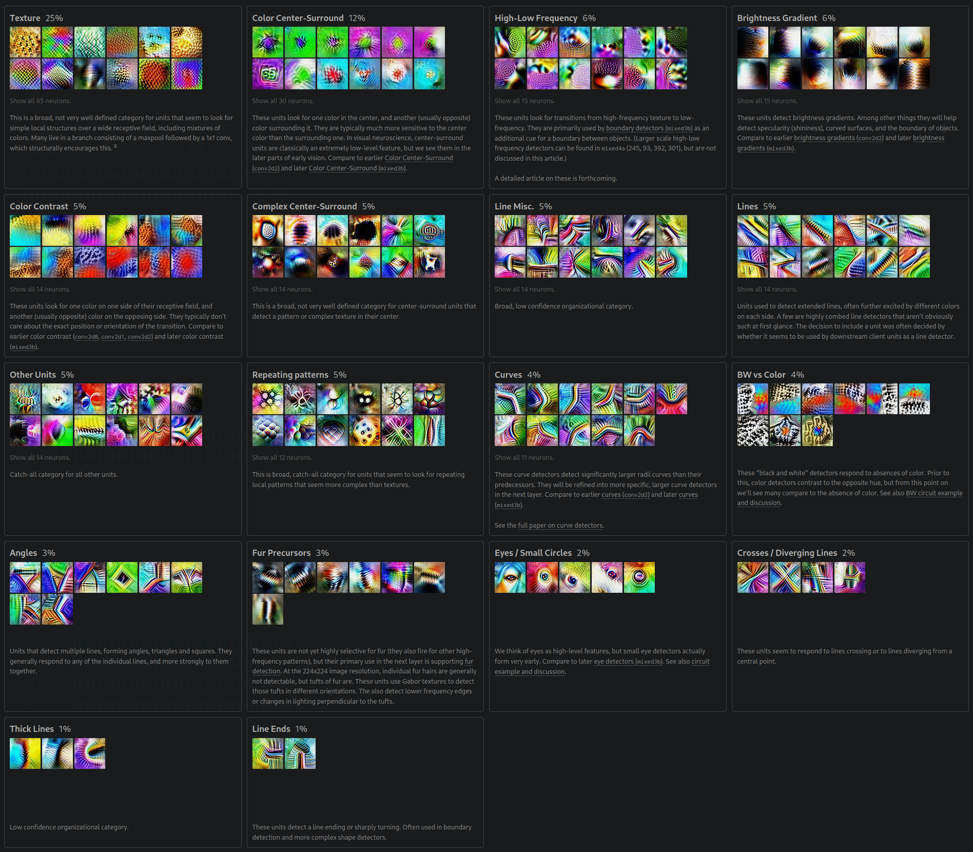
Here are some filters that appear in the second layer of InceptionV1:

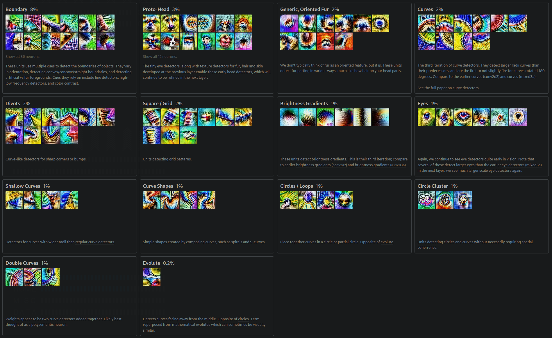
In the third convolutional layer, we find some more complex filters:

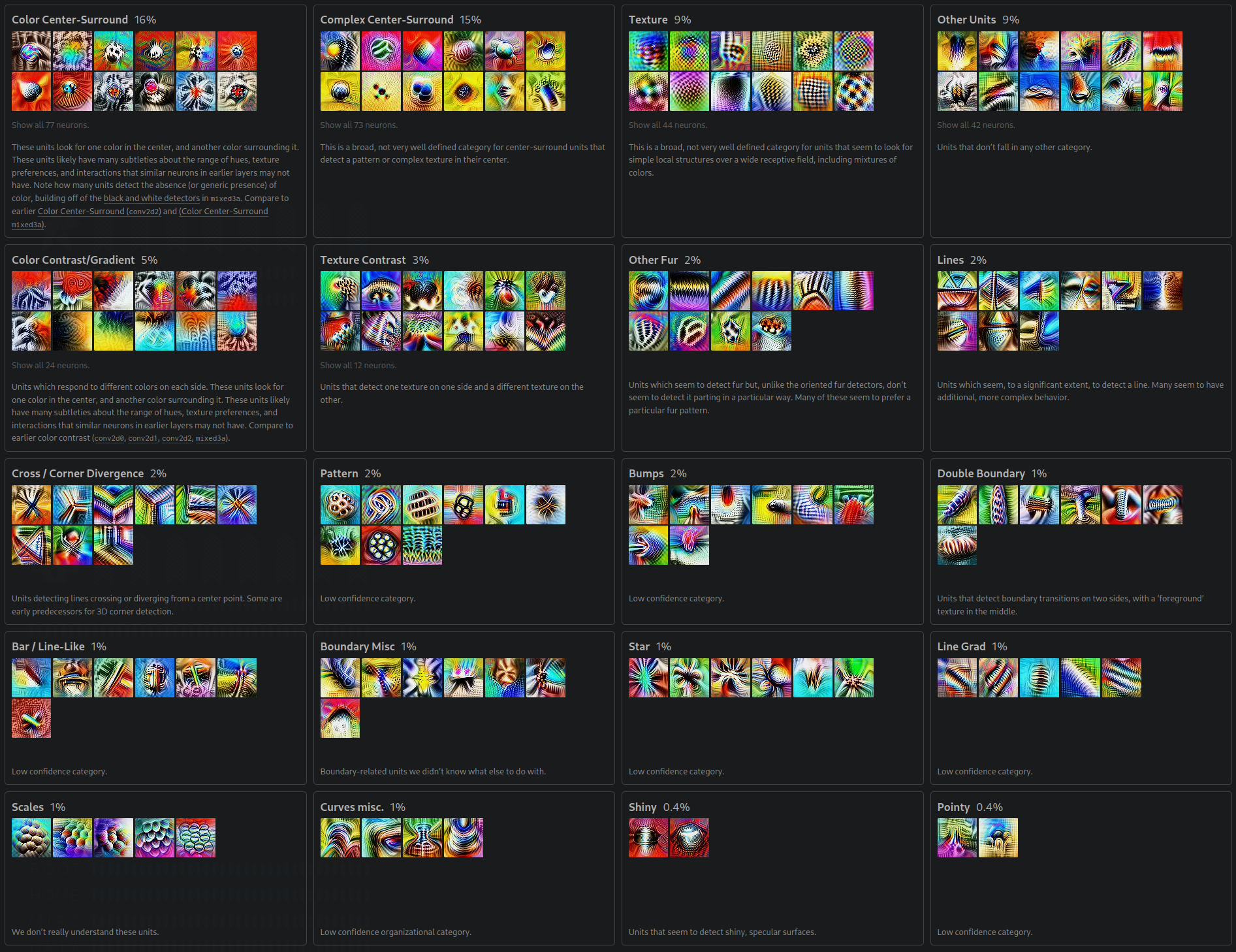
The fourth layer becomes exotic, with pretty colors and we even begin to see what look like early fur, eye, and even head detectors.

If you would like to explore more feature visualizations from a wide range of vision models trained on several datasets, check out OpenAI's Microscope project.