
Multihead Attention
[In progress] Implementing Multi-Head Attention and Optimized Matrix Multiplication via Strassen's Algorithm.


Before we get started I have to apologize: firstly for the pun (there are only so many Multi-Head Attention puns available) and secondly for getting nerd sniped once again – I'll finish up the compiler series soon enough I promise.
We may be standing at the single greatest lever point in human history. As cliche as it sounds I fundamentally believe that the repercussions of AI on society will rival the internet before it's all said and done. If computers are bicycles for the mind, Deep Learning methods are performance enhancing drugs – the average person now becomes Lance Armstrong. The Machine Learning industry has had a seasonal past. Public sentiment has oscillated between "the machines will kill us all" and "AI is a pipe dream". We're currently in the heat of an AI summer, thanks to consumer facing products such as ChatGPT, and the robust developer ecosystem that has developed around Natural Language Processing, Image Classification and Generation, etc. I believe that we're at an inflection point in the pace of development, accelerating towards the singularity.
"Midas was wrong, everything we touch turns to silicon"
- George Hotz
But I digress, enough of the melodrama – let's get down to the nitty gritty. For the sake of precision, let's get some terminology out of the way. I've been using AI, Machine Learning, and Deep Learning interchangeably so far. There is a distinction between them though:
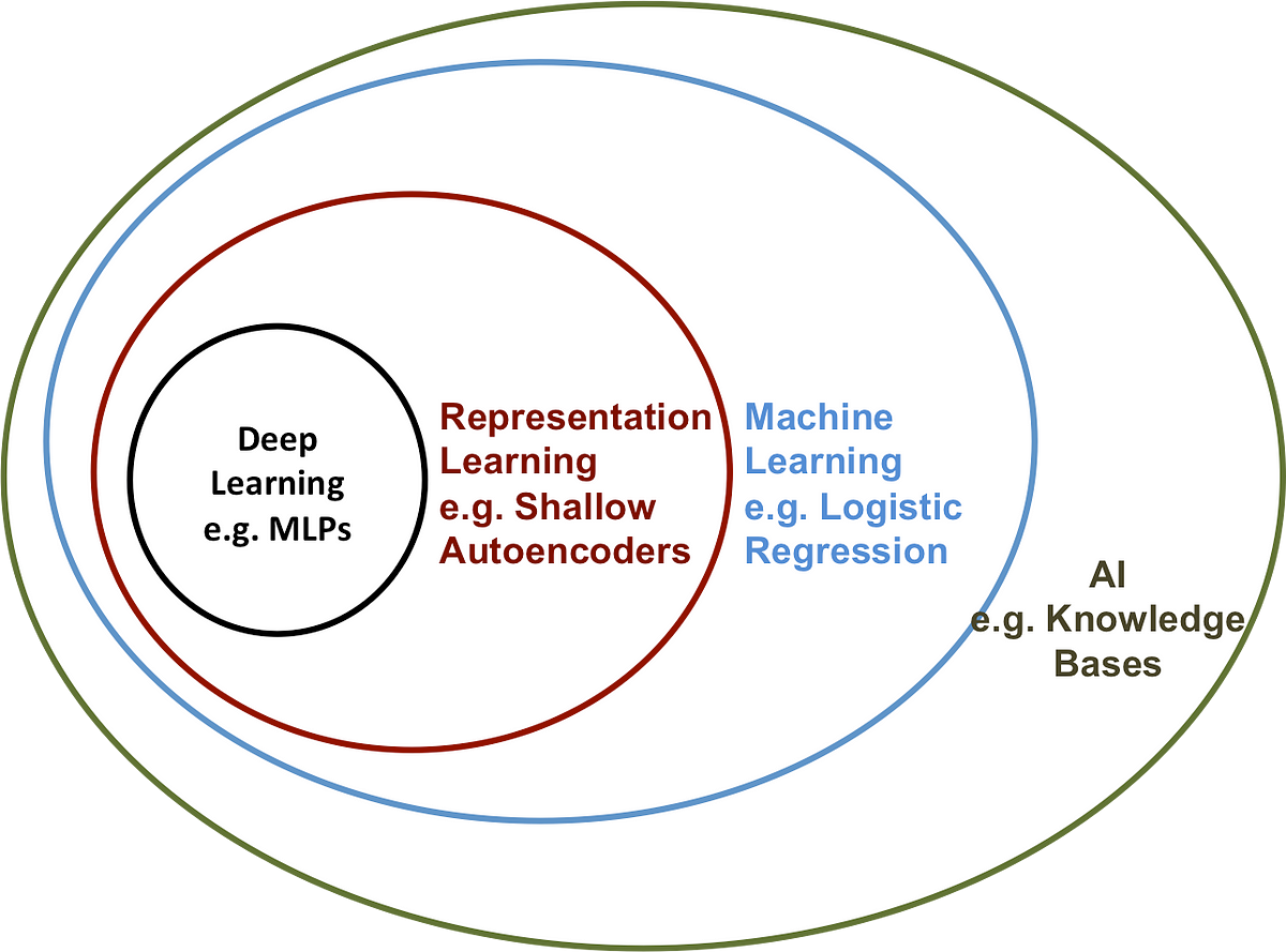
From here on out I'll focus on Deep Learning as that is where most of the recent progress has been made. It's important to emphasize that Deep Learning is not a silver bullet, depending on the context, Machine Learning methods may be much more efficient or preferable. For example, despite all the exotic new Deep Learning architectures, banks still use Decision Forests and the like to determine whether to loan an individual money. Due to regulations, they have to be able to explain why an individual was turned down. Neural Networks (Deep Learning) are often thought of as "black boxes" and lack the level of interpretability necessary.
The seed that sparked the recent hype around the space was the advent of the Transformer architecture as described in Attention is All You Need. Transformers first saw rapid and extensive adoption in the Natural Language Processing space, secondly in Computer Vision, and have shot out from there. While we won't dive into the transformer architecture – you'd be better off just reading the paper for that – we will try to give a thorough treatment to the attention mechanism. and try to implement something similar to how it looks behind the scenes.
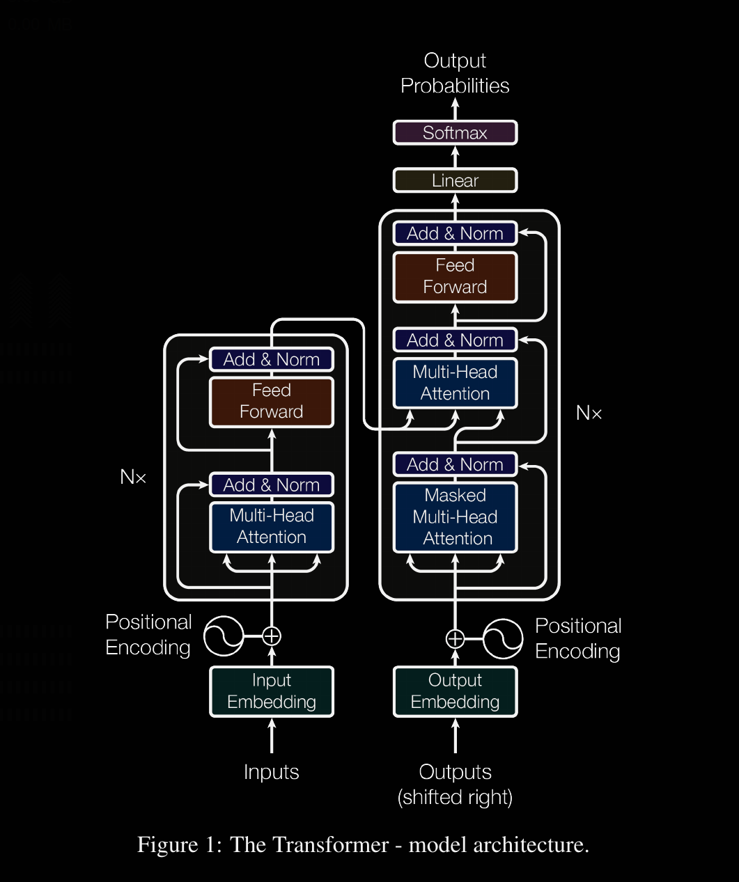
The Transformer is a magnificient neural network architecture because it is a general-purpose differentiable computer. It is simultaneously:
— Andrej Karpathy (@karpathy) October 19, 2022
1) expressive (in the forward pass)
2) optimizable (via backpropagation+gradient descent)
3) efficient (high parallelism compute graph)
Attention: The Secret Sauce
As previously noted by Phil Karlton, one of the hardest problems in Computer Science is naming things. The Attention mechanism is aptly named. Attention in the context of Deep Learning closely mirrors our every day meaning of the word. It allows a system to keep both previous input and previous output in context when generating new output. Furthermore, through training a Transformer model, the model learns how to rank the components of a state's context in terms of relevance when predicting the next word or token. Take, for example, a sentence like "My dog hardly ate today, I hope he isn't sick." If we couldn't confidently reference the past context, we'd be stumped. Who is "he"? What makes you think "he" might be sick? Long range dependencies are key to understanding the meaning and structure of language and then acting on that understanding (e.g. through response or translation) in a human-like fashion.
Machine Learning allows us to learn from and make actionable conclusions based on real world data. Just as Physics describes formulas that represent reality and can be used to predict future states of a given physical system, Machine Learning practitioners believe that many real-world systems subscribe to similar mappings from input to output. Often times these functions are too complex to be determined analytically, but as determined by the Universal Approximation Theorem, Neural Networks are capable of approximating any function to arbitrary precision.
Linear Algebra plays a fundamental role in Machine Learning systems. The goal of ML is to approximate and exploit the intrinsic low-rank feature spaces of a given data set. Let's simplify that statement a bit. We gather high dimensional, noisy data. Then try to the best way to determine and represent what the defining pattern is. To reference Nate Silver's book, we are looking for "the signal in the noise". Having a good intuition for vector spaces, matrices as linear transformations and change of basis is invaluable for understanding these systems. Each ML algorithm has a different way of finding optimal embeddings for the data that are both informative and interpretable. These optimal embeddings are represented by matrices. In Deep Learning, Neural Networks are composed of several layers of Neurons. Each Layer is represented by a matrix. In Deep Learning, the internal layers are often referred to as hidden states. The elements of our hidden state matrices are called weights and they are iteratively learned by our model.
Recurrent Neural Networks were the previous state of the art approach to the NLP space. RNNs used sequential methods to gather the context of a given state. An input sequence was processed incrementally according to the order of words in the sequence. Hidden states are computed recursively – each hidden state is generated as a function of the previous hidden state and the input for the given position. While recursion often provides elegant looking solutions, they can easily pollute the stack through nested function calls. This puts a hard cap on the size of the input sequences, quickly bottlenecking on the size of one's memory since we are often operating on large matrices.
The beauty of GPUs is that they are massively parallel machines that are optimized to perform matrix multiplication. A crude simplification of Deep Learning is that it is a way of brute forcing matrix multiplications to solve an optimization problem. It is this very parallelism is what gave rise to the field of Deep Learning in the first place. As I previously stated, with the end of Dennard Scaling and Moore's Law, we can no longer rely on regular improvements in clock speeds to improve our programs performance for us. The future of speedups will likely have to come from improvements in architecture and parallelism.
"The biggest lesson that can be read from 70 years of AI research is that general methods that leverage computation are ultimately the most effective, and by a large margin."
- Richard Sutton
The parallelizability of the Attention architecture is precisely what brought Transformers to the forefront. [WRITE ABOUT WHY PARALLELIZABLE COMPARED TO RNN] First things first let's introduce the attention function. An attention function is a mapping of a query vector (Q) and a set of Key/Value pair vectors (K, V) to an output vector. [We will ignore how the input vectors are encoded, as this is arbitrary.] There are multiple variants, but we will focus on a variant of dot-product attention since the dot product operation is fast and space-efficient.
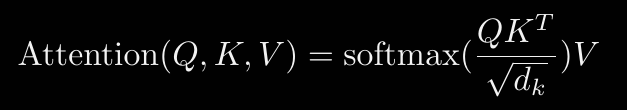
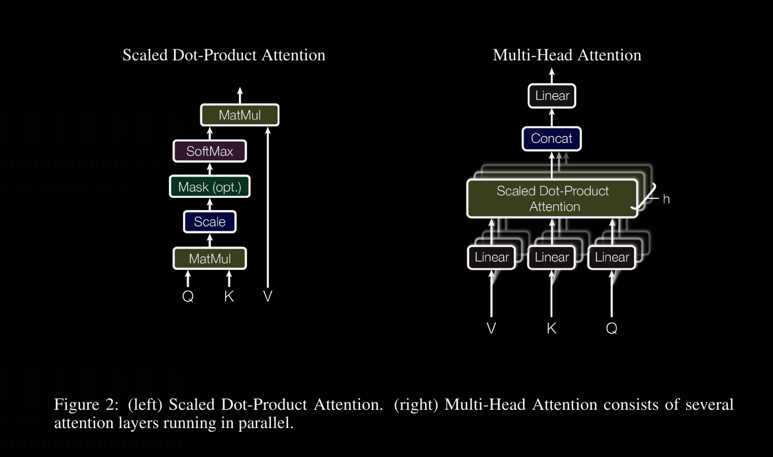
- We multiply the Query vector with the Key vector
- Scale the resulting matrix element-wise by a factor of 1/√ d_k (note: d_k = the size of the key vector – done for numerical reasons)
- Perform softmax on resulting matrix
- Then multiply the softmax matrix by the Value vector
First step to computing the output is to multiply the query vector with the key vector. The postscript "T" represents the transpose operation in which a matrices rows are interchanged with its columns. In the case of a vector, a row vector (1 x N) becomes a column vector (N x 1). This is done because matrix multiplication follows stricter rules than scalar multiplication. The second matrix must have the same number of rows as the first matrix has columns. Consequently, order matters – A x B often does not equal B x A. The product of an MxK matrix with an KxN matrix results in an MxN matrix. The ij_th component of the product matrix is computed by the sum of element wise product of the i_th row of the first matrix with the j_th column of the second matrix. In the case of multi-head attention, several query vectors are concatenated to get a query matrix, and likewise with their respective corresponding key vectors. The number of examples that are grouped into matrices together is your batch size.
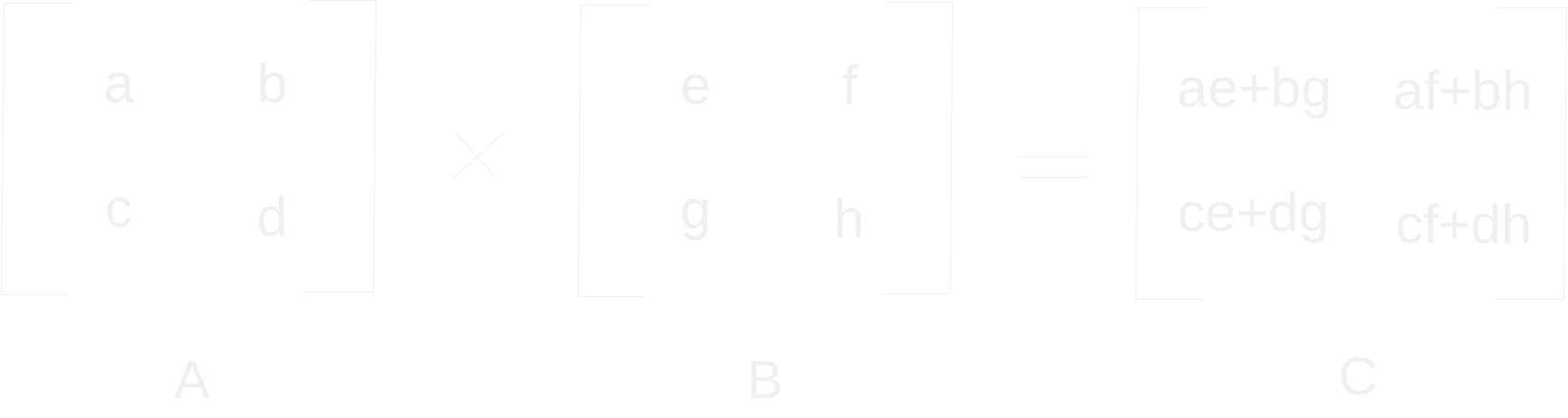
Let's talk about the computational complexity of matrix multiplication as described above. Big-O notation is a way to describe how well computations scale in terms of their input. In the example above we have two 2x2 matrices – let n = 2. To compute the matrix-product we have to perform 8 scalar multiplications and 4 scalar additions. Or, as a function of the input size – n3 scalar multiplications and n3 - n2 scalar additions. In big-O notation, we focus on dominating terms, since scalar multiplications are more computationally expensive, we say this way of performing matrix multiplication is O(n3). This is quickly apparent when looking at a code sample. We have three for loops whose number of iterations is contingent on the matrix's size.
def matmul(C, A, B):
	for m in range(C.rows):
    		for k in range(A.cols):
        		for n in range(C.cols):
            			C[m, n] += A[m, k] * B[k, n]
Let's take a step back and think about what the connection is between matrix multiplication and context. How would you contextualize some ordered set of numbers (e.g. 2, 4, 6, 8, 10) to guess what the next one would be? One idea is to use a series of averages as a hint on what to guess. First, let's split our set into several of it's subsets so that we have several examples to work off of. Our examples of [input] -> [next element] would be: [2] -> [4], [2, 4] -> [6], [2, 4, 6] -> [8], and [2, 4, 6, 8] -> [10]. If we didn't have the human intuition to recognize that we're dealing with the set of even integers, we could notice that so far the pattern seems to be: calculate the average value, then multiply it by two to get the next character. That's a reliable pattern that effectively compresses the underlying distribution down to a simple rule. As I'm sure you've noticed, this is definitely a lossy compression, as the average only conveys so much information about the previous elements. But still, a compression nonetheless.
The key to the self-attention mechanism is the extension of this idea: thinking of matrices as weighted aggregations. Let's take a lower triangular matrix 3x3 filled with ones on and below the diagonal. Then multiply it with another 3x3 matrix.
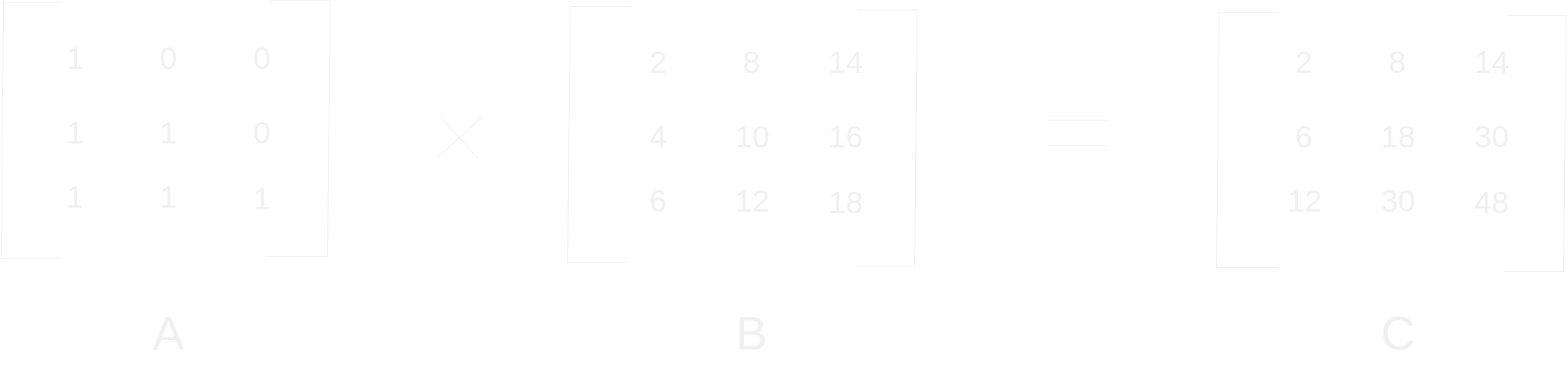
As you can see, this operation sums the elements of each column, going from top to bottom. We can combine this with normalizing across the rows of A (dividing such that each row sums to 1) to get an moving average as you go down the columns of B.
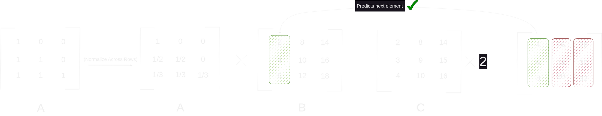
In Transformer networks, we use the matrix A as our set of weights. To avoid wasting compute cycles when training our model, we have to think of a way to intelligently initialize the weights.
tril = torch.tril(torch.ones(N,N)) # Creates a lower triangular matrix (size = NxN) with ones on and below diagonal
weights = torch.zeros((N,N)) # initialize weights to zeros
weights = weights.masked_full(tril == 0, float('-inf')) # In all positions where tril = 0 (above diagonal), set the corresponding location on weights to negative infinity
weights = F.softmax(weights, dim=-1) # perform softmax across the rows of weights
Although this seems like an overly complex way to initialize the weights, we do it this way to ensure that future tokens in a sequence have no impact on the current token we are predicting. Then, through autodifferentiation (AD), we can iteratively tune the weights in search an optimal compression of our input that can then be scaled, fed into a softmax, and multiplied once again to provide a good probability distribution to make predictions using our trained model. These predictions are what we use to evaluate loss. If we just used `torch.tril(torch.ones(N,N))` to initialize the weights, then we would have zeros above the diagonal. Those could potentially be nudged during AD and affect our predictions which doesn't make sense and isn't what we want.
Most examples of matrix multiplication that we can wrap our heads around are trivial in size to a computer. But imagine what happens when we're dealing with realistic matrices? Take the average computer monitor resolution of 1920 pixels wide by 1080 pixels high and represent is as an 1920 x 1080 matrix. The number of elements (pixels) is just over 2 million – for a grayscale image. If we want an RGB image that number grows to over 6 million. Now let's imagine that we want to train a computer vision model and want to train on a modern dataset (e.g JFT-300M that the original Vision Transformer ViT was trained on) and multiply that number by 300 million. We're at ~1.8e15 elements. Then we have to perform an untold number of multiplications on each matrix.
We have to find ways to improve the tractability of training such a model. There are a few things we can do: we can compress the images, choose a parallelizable architecture like the transformer, and we can also look for ways to more efficiently perform each matrix multiplication. Let's focus on the latter
Before getting into more exotic optimized matrix multiplication algorithms, let's first take a quick look at the language we are using. Python is a great language, especially for developer productivity. Often times that's the real bottleneck: first, ones focus should be on just getting a minimum viable product out as fast as possible. Once we have something that works, we can deploy it into production. It's only then that we should optimize, refine, and iterate on our code. As Tony Hoare said: "premature optimization is the root of all evil in programming." One of the main areas where Python struggles is in performance. Whenever we need the utmost performance, we often want to reach for a systems programming language like Rust :). But then, we lose the developer friendliness of Python :/. If only there were a middle ground.
Enter Mojo – a programming language that "combines the usability of Python with the performance of C". Mojo is a new language by Chris Lattner (creator of Swift, LLVM, etc.). A brief disclaimer is necessary: Mojo, a superset of Python with seamless interop, is in early development at the time of writing, and is not ready for production. Some cool features that Mojo has are: progressive types, zero cost abstractions, ownership & borrow checker (makes me smile as a part time Rustacean), portable parametric algorithms, language integrated auto-tuning. Check out this link to see how switching to Mojo for matrix multiplications can lead to a speedup of 17.5x (and up to 14,050x if you optimize the heck out of it). Chris Lattner is a really smart guy, and as a person somewhat interested in programming language design and compilers I think this is a cool project worth checking out.
Because the reader is more likely to be familiar with Python, we'll just focus on improving the algorithm itself.
How are matrix multiplications actually implemented in practice?
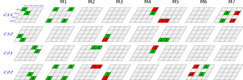
The first big advancement to efficient matrix multiplication came in 1969 from Volker Strassen. The algorithm Strassen devised is much more complicated (to us humans) than the naive algorithm. Strassen took more of a divide and conquer approach, recursively partitioning the factor matrices and processing those partitions. Let's take a look at the 2x2 case. Take the same two matrices A and B as we saw above. Instead of going row by row, we are going to partition A, B, and the product matrix C into equally sized square sub-matrices, padding with zeros if the size is an odd number. We partition recursively until each sub-matrix contains a single element. In each subroutine we initialize 7 intermediate matrices, then use them to define the corresponding product sub-matrix. This process is looped until we end up with the correctly sized product matrix.
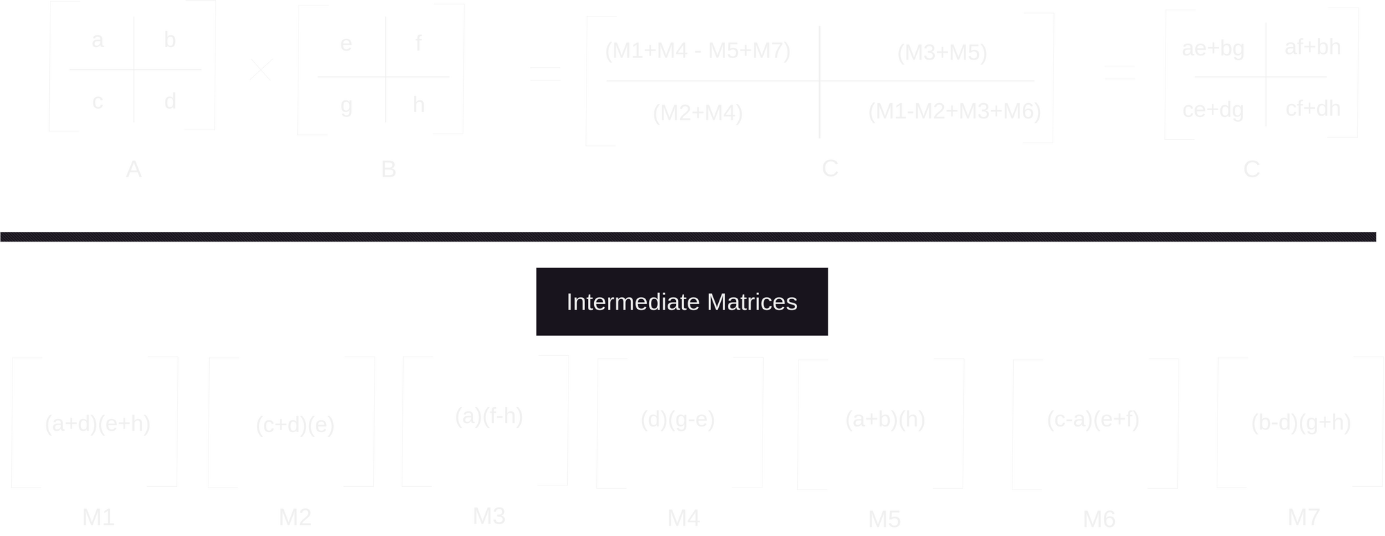
Ok, that was a lot. The reader can verify that the solutions are equivalent. The important takeaway is that we now only have 7 multiplications instead of 8. I know we introduced a ton of additions, but remember, we only care about the number of multiplications. This may not seem like a big deal, but it really adds up when dealing with large matrices. In terms of complexity we move from O(n3) to O(nlog_2(7)) or ~ O(n2.807). For the 2x2 case, we dealt with 1 x 1, single element sub-matrices. What if, we're trying to multiply an 8x8? Well, we would have sub-matrices of size 2x2. Then for each sub-matrix, we just do the same process of breaking it down into sub-matrices and calculating each element. Isn't that beautiful? There's something really elegant and pleasing about recursive algorithms. I think it's the same self-referential nature that also makes fractals and inductive proofs especially nice.
So, what does this look like in Python?
Links for future reference: